The GPU's specialty, and by extension OpenGL's, is in rendering three-dimensional scenes. If you compare last chapter's hello-gl program to, say, Crysis, you might notice that our demo is missing one of those dimensions (among other things). In this chapter, I'm going to fix that. We'll cover the basic math that makes 3d rendering happen, looking at how transformations are done using matrices and how perspective projection works. Wikipedia does a great job going in-depth about the algorithmic details, so I'm going to spend most of my time talking at a high level about what math we use and why, linking to the relevant Wikipedia articles if you're interested in exploring further. As we look at different transformations, we're going to take the vertex shader from last chapter and extend it to implement those transformations, animating the "hello world" image by moving its rectangle around in 3d space.
Before we start, there are some changes we need to make to last chapter's hello-gl program so that it's easier to play around with. These changes will allow us to write different vertex shaders and supply them as command-line arguments when we run the program, like so:
./hello-gl hello-gl.v.glsl
You can pull these changes from my hello-gl-ch3 github repo.
We'll start by expanding our vertex array to hold three-dimensional vectors. We'll actually pad them out to four components—the fourth component's purpose will become clear soon. For now, we'll just set all the fourth components to one. Let's update our vertex array data in hello-gl.c:
static const GLfloat g_vertex_buffer_data[] = {
    -1.0f, -1.0f, 0.0f, 1.0f,
     1.0f, -1.0f, 0.0f, 1.0f,
    -1.0f,  1.0f, 0.0f, 1.0f,
     1.0f,  1.0f, 0.0f, 1.0f
};
and our glVertexAttribPointer call:
    glVertexAttribPointer(
        g_resources.attributes.position,  /* attribute */
        4,                                /* size */
        GL_FLOAT,                         /* type */
        GL_FALSE,                         /* normalized? */
        sizeof(GLfloat)*4,                /* stride */
        (void*)0                          /* array buffer offset */
    );
When we start transforming our rectangle, it will no longer completely cover the window, so let's add a glClear to our render function so we don't get garbage in the background. We'll set it to dark grey so it's distinct from the black background of our images:
static void render(void)
{
    glClearColor(0.1f, 0.1f, 0.1f, 1.0f);
    glClear(GL_COLOR_BUFFER_BIT);
    /* ... */
}
Now let's generalize a few things. First, we'll change our uniform state to include GLUT's timer value directly rather than the fade_factor precalculated. This will let our new vertex shaders perform additional time-based effects.
static void update_timer(void)
{
    int milliseconds = glutGet(GLUT_ELAPSED_TIME);
    g_resources.timer = (float)milliseconds * 0.001f;
    glutPostRedisplay();
}
You'll also have to search-and-replace all of the other references to fade_factor with timer. Once that's done, we'll change our main and make_resources functions so they can take the vertex shader filename as an argument. This way, we can easily switch between the different vertex shaders we'll be writing:
static int make_resources(const char *vertex_shader_file)
{
    /* ... */
    g_resources.vertex_shader = make_shader(
        GL_VERTEX_SHADER,
        vertex_shader_file
    );
    /* ... */
}
int main(int argc, char** argv)
{
    /* ... */
    if (!make_resources(argc >= 2 ? argv[1] : "hello-gl.v.glsl")) {
        fprintf(stderr, "Failed to load resources\n");
        return 1;
    }
    /* ... */
}
Now let's update our shaders to match our changes to the uniform state and vertex array. We can move the fade factor calculation into the vertex shader, which will pass it on to the fragment shader as a varying value. In hello-gl.v.glsl:
#version 110

uniform float timer;

attribute vec4 position;

varying vec2 texcoord;
varying float fade_factor;

void main()
{
    gl_Position = position;
    texcoord = position.xy * vec2(0.5) + vec2(0.5);
    fade_factor = sin(timer) * 0.5 + 0.5;
}
A new feature of GLSL I use here is vector swizzling: not only can you address the components of a vec type as if they were struct fields by using .x, .y, .z, and .w for the first through fourth components, you can also string together the element letters to collect multiple components in any order into a longer or shorter vector type. position.xy picks out as a vec2 the first two elements of our now four-component position vector. We can then feed that vec2 into the calculation for our texcoord, which remains two components long.
Finally, in hello-gl.f.glsl, we make fade_factor assume its new varying identity:
#version 110

uniform sampler2D textures[2];

varying float fade_factor;
varying vec2 texcoord;

void main()
{
    gl_FragColor = mix(
        texture2D(textures[0], texcoord),
        texture2D(textures[1], texcoord),
        fade_factor
    );
}
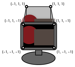
The destination space for the vertex shader, which I've been informally referring to as "screen space" in the last couple of chapters, is more precisely called projection space. The visible part of projection space is the unit-radius cube from (–1, –1, –1) to (1, 1, 1). Anything outside of this cube gets clipped and thrown out. The x and y axes map across the viewport, the part of the screen in which any rendered output will be displayed, with (–1, –1, z) corresponding to the lower left corner, (1, 1, z) to the upper right, and (0, 0, z) to the center. The rasterizer uses the z coordinate to assign a depth value to every fragment it generates; if the framebuffer has a depth buffer, these depth values can be compared against the depth values of previously rendered fragments, allowing parts of newly-rendered objects to be hidden behind objects that have already been rendered into the framebuffer. (x, y, –1) is the near plane and maps to the nearest depth value. At the other end, (x, y, 1) is the far plane and maps to the farthest depth value. Fragments with z coordinates outside of that range get clipped against these planes just like they do the edges of the screen.
Projection space is computationally convenient for the GPU, but it's not very usable by itself for modeling vertices within a scene. Rather than input projection-space vertices directly to the pipeline, most programs use the vertex shader to project objects into it. The pre-projection coordinate system used by the program is called world space, and can be moved, scaled, and rotated relative to projection space in whatever way the program needs. Within world space, objects also need to move around, changing position, orientation, size, and shape. Both of these operations, mapping world space to projection space and positioning objects in world space, are accomplished by performing transformations with mathematical structures called matrices.
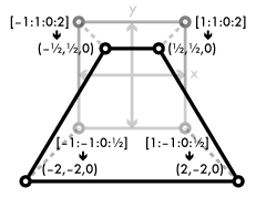
Linear transformations are operations on an object that preserve the relative size and orientation of parts within the object while uniformly changing its overall size or orientation. They include rotation, scaling, and shearing. If you've ever used the "free transform" tool in Photoshop or GIMP, these are the sorts of transformations it performs. You can think of a linear transformation as taking the x, y, and z axes of your coordinate space and mapping them to a new set of arbitrary axes x', y', and z':
For clarity, the figure is two-dimensional, but the same idea applies to 3d. To represent a linear transformation numerically, we can take the vector values of those new axes and arrange them into a 3×3 matrix. We can then perform an operation called matrix multiplication to apply a linear transformation to a vector, or to combine two transformations into a single matrix that represents the combined transformation. In standard mathematical notation, matrices are represented so that the axes are represented as columns going left-to-right. In GLSL and in the OpenGL API, matrices are represented as an array of vectors, each vector representing a column in the matrix. In source code, this results in the values looking transposed from their mathematical notation. This is called column-major order (as opposed to row-major order, in which each vector element of the matrix array would be a row of the matrix). GLSL provides 2×2, 3×3, and 4×4 matrix types named mat2 through mat4. It also overloads its multiplication operator for use between matn values of the same type, and between matns and vecns, to perform matrix-matrix and matrix-vector multiplication.
A nice property of linear transformations is that they work well with the rasterizer's linear interpolation. If we transform all of the vertices of a triangle using the same linear transformation, every point on its surface will retain its relative position to the vertices, so textures and other varying values will transform with the vertices they fill out.
Note that all linear transformations occur relative to the origin, that is, the (0, 0, 0) point of the coordinate system, which remains constant through a linear transformation. Because of this, moving an object around in space, called translation in mathematical terms, is not a linear transformation, and cannot be represented with a 3×3 matrix or composed into other 3×3 linear transform matrices. We'll see how to integrate translation into transformation matrices shortly. For now, let's try some linear transformations:
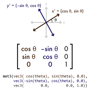
We'll start by writing a shader that spins our rectangle around the z axis. Using the timer uniform value as a rotation angle, we'll construct a rotation matrix, using the sin and cos functions to rotate our matrix axes around the unit circle. The shader looks like this; it's in the repo as rotation.v.glsl:
#version 110

uniform float timer;

attribute vec4 position;

varying vec2 texcoord;
varying float fade_factor;

void main()
{
    mat3 rotation = mat3(
        vec3( cos(timer),  sin(timer),  0.0),
        vec3(-sin(timer),  cos(timer),  0.0),
        vec3(        0.0,         0.0,  1.0)
    );
    gl_Position = vec4(rotation * position.xyz, 1.0);
    texcoord = position.xy * vec2(0.5) + vec2(0.5);
    fade_factor = sin(timer) * 0.5 + 0.5;
}
(I'm going to be listing only the main function of the next few shaders; the uniform, attribute, and varying declarations will all remain the same from here.) With our changes to hello-gl we can run it like so:
./hello-gl rotation.v.glsl
And this is the result:
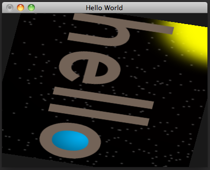
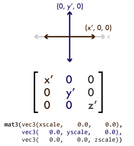
You probably noticed that the rectangle appears to be horizontally distorted as it rotates. This is because our window is wider than it is tall, so the screen distance covered along a unit on the x axis of projection space is longer than the distance the same unit would cover along the y axis. The window is 400 pixels wide and 300 pixels high, giving it an aspect ratio of 4:3 (the width divided by the height). (This will change if we resize the window, but we won't worry about that for now.) We can compensate for this by applying a scaling matrix that scales the x axis by the reciprocal of the aspect ratio, as in window-scaled-rotation.v.glsl:
    mat3 window_scale = mat3(
        vec3(3.0/4.0, 0.0, 0.0),
        vec3(    0.0, 1.0, 0.0),
        vec3(    0.0, 0.0, 1.0)
    );
    mat3 rotation = mat3(
        vec3( cos(timer),  sin(timer),  0.0),
        vec3(-sin(timer),  cos(timer),  0.0),
        vec3(        0.0,         0.0,  1.0)
    );
    gl_Position = vec4(window_scale * rotation * position.xyz, 1.0);
    texcoord = position.xy * vec2(0.5) + vec2(0.5);
    fade_factor = sin(timer) * 0.5 + 0.5;
 Note that the order in which we rotate and scale is important. Unlike scalar multiplication, matrix multiplication is noncommutative: Changing the order of the arguments gives different results. This should make intuitive sense: "rotate an object, then squish it horizontally" gives a different result from "squish an object horizontally, then rotate it". As matrix math, you write transformation sequences out right-to-left, backwards compared to English: scale * rotate * vector rotates the vector first, whereas rotate * scale * vector scales first.
Now that we've compensated for the distortion of our window's projection space, we've revealed a dirty secret. Our input rectangle is really a square, and it doesn't match the aspect ratio of our image, leaving it scrunched. We need to scale it again outward, this time before we rotate, as in window-object-scaled-rotation.v.glsl:
    mat3 window_scale = mat3(
        vec3(3.0/4.0, 0.0, 0.0),
        vec3(    0.0, 1.0, 0.0),
        vec3(    0.0, 0.0, 1.0)
    );
    mat3 rotation = mat3(
        vec3( cos(timer),  sin(timer),  0.0),
        vec3(-sin(timer),  cos(timer),  0.0),
        vec3(        0.0,         0.0,  1.0)
    );
    mat3 object_scale = mat3(
        vec3(4.0/3.0, 0.0, 0.0),
        vec3(    0.0, 1.0, 0.0),
        vec3(    0.0, 0.0, 1.0)
    );
    gl_Position = vec4(window_scale * rotation * object_scale * position.xyz, 1.0);
    texcoord = position.xy * vec2(0.5) + vec2(0.5);
    fade_factor = sin(timer) * 0.5 + 0.5;
(Alternately, we could change our vertex array and apply a scaling transformation to our generated texcoords. But I promised we wouldn't be changing the C anymore in this chapter.)
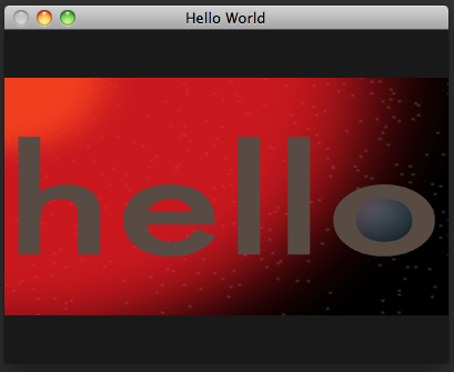
With this shader, our rectangle now rotates the way we would expect it to: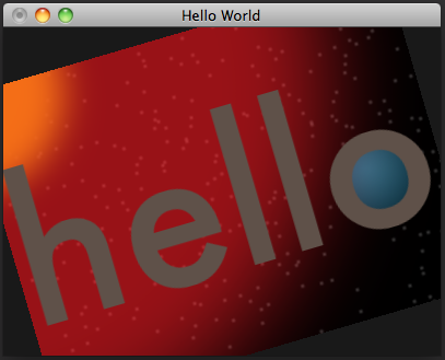
The window_scale matrix conceptually serves a different purpose from the rotation and object_scale matrices. While the latter two matrices set up our input vertices to be where we want them in world space, the window_scale serves to project world space into projection space in a way that gives an undistorted final render. Matrices used to orient objects in world space, like our rotation and object_scale matrices, are called model-view matrices, because they are used both to transform models and to position them relative to the viewport. The matrix we use to project, in this case window_scale, is called the projection matrix. Although both kinds of matrix behave the same, and the line drawn between them is mathematically arbitrary, the distinction is useful because a 3d application will generally only need a few projection matrices that change rarely (usually only if the window size or screen resolution changes). On the other hand, there can be countless model-view matrices for all of the objects in a scene, which will update constantly as the objects animate.
Projecting with a scaling matrix, as we're doing here, produces an orthographic projection, in which objects in 3d space are rendered at a constant scale regardless of their distance from the viewport. Orthographic projections are useful for rendering two-dimensional display elements, such as the UI controls of a game or graphics tool, and in modeling applications where the artist needs to see the exact scales of different parts of a model, but they don't adequately present 3d scenes in a way most viewers expect. To demonstrate this, let's break out of the 2d plane and alter our shader to rotate the rectangle around the x axis, as in orthographic-rotation.v.glsl:
    const mat3 projection = mat3(
        vec3(3.0/4.0, 0.0, 0.0),
        vec3(    0.0, 1.0, 0.0),
        vec3(    0.0, 0.0, 1.0)
    );

    mat3 rotation = mat3(
        vec3(1.0,         0.0,         0.0),
        vec3(0.0,  cos(timer),  sin(timer)),
        vec3(0.0, -sin(timer),  cos(timer))
    );
    mat3 scale = mat3(
        vec3(4.0/3.0, 0.0, 0.0),
        vec3(    0.0, 1.0, 0.0),
        vec3(    0.0, 0.0, 1.0)
    );
    gl_Position = vec4(projection * rotation * scale * position.xyz, 1.0);
    texcoord = position.xy * vec2(0.5) + vec2(0.5);
    fade_factor = sin(timer) * 0.5 + 0.5;
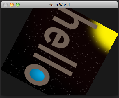
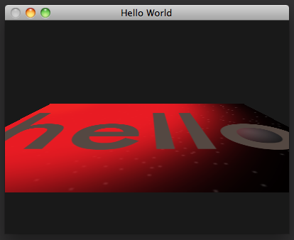
With an orthographic projection, the rectangle doesn't very convincingly rotate in 3d space—it just sort of accordions up and down. This is because the top and bottom edges of the rectangle remain the same apparent size as they move toward and away from the view. In the real world, objects appear smaller in our field of view proportional to how far from our eyes they are. This effect is called perspective, and transforming objects to take perspective into account is called perspective projection. Perspective projection is accomplished by shrinking objects proportionally to their distance from the "eye". An easy way to do this is to divide each point's position by some function of its z coordinate. Let's arbitrarily decide that zero on the z axis remains unscaled, and that points elsewhere on the z axis scale by half their distance from zero. Correspondingly, let's also scale the z axis by half, so that the end of the rectangle coming toward us doesn't get clipped to the near plane as it gets magnified. We'll end up with the shader code in naive-perspective-rotation.v.glsl:
    const mat3 projection = mat3(
        vec3(3.0/4.0, 0.0, 0.0),
        vec3(    0.0, 1.0, 0.0),
        vec3(    0.0, 0.0, 0.5)
    );

    mat3 rotation = mat3(
        vec3(1.0,         0.0,         0.0),
        vec3(0.0,  cos(timer),  sin(timer)),
        vec3(0.0, -sin(timer),  cos(timer))
    );
    mat3 scale = mat3(
        vec3(4.0/3.0, 0.0, 0.0),
        vec3(    0.0, 1.0, 0.0),
        vec3(    0.0, 0.0, 1.0)
    );

    vec3 projected_position = projection * rotation * scale * position.xyz;
    float perspective_factor = projected_position.z * 0.5 + 1.0;

    gl_Position = vec4(projected_position/perspective_factor, 1.0);
    texcoord = position.xy * vec2(0.5) + vec2(0.5);
    fade_factor = sin(timer) * 0.5 + 0.5;

Now the overall shape of the rectangle appears to rotate in perspective, but the texture mapping is all kinky. This is because perspective projection is a nonlinear transformation—different parts of the rectangle get scaled differently depending on how far away they are. This interferes with the linear interpolation the rasterizer applies to the texture coordinates across the surface of our triangles. To properly project texture coordinates as well as other varying values in perspective, we need a different approach that takes the rasterizer into account.
Directly applying perspective to an object may not be a linear transformation, but the divisor that perspective applies is a linear function of the perspective distance. If we stored the divisor out-of-band as an extra component of our vectors, we could apply perspective as a matrix transformation, and the rasterizer could linearly interpolate texture coordinates correctly before the perspective divisor is applied. This is in fact what that mysterious 1.0 we've been sticking in the fourth component of our vectors is for. The projection space that gl_Position addresses uses homogeneous coordinates. That fourth component, labeled w, divides the x, y, and z components when the coordinate is projected. In other words, the homogeneous coordinate [x:y:z:w] projects to the linear coordinate (x/w, y/w, z/w).
With this trick, we can construct a perspective matrix that maps distances on the z axis to scales on the w axis. As I mentioned, the rasterizer also interpolates varying values in homogeneous space, before the coordinates are projected, so texture coordinates and other varying values will blend correctly over perspective-projected triangles using this matrix. The 3×3 linear transformation matrices we've covered extend to 4×4 easily—just extend the columns to four components and add a fourth column that leaves the w axis unchanged. Let's update our vertex shader to use a proper perspective matrix and mat4s to transform our rectangle, as in perspective-rotation.v.glsl:
    const mat4 projection = mat4(
        vec4(3.0/4.0, 0.0, 0.0, 0.0),
        vec4(    0.0, 1.0, 0.0, 0.0),
        vec4(    0.0, 0.0, 0.5, 0.5),
        vec4(    0.0, 0.0, 0.0, 1.0)
    );

    mat4 rotation = mat4(
        vec4(1.0,         0.0,         0.0, 0.0),
        vec4(0.0,  cos(timer),  sin(timer), 0.0),
        vec4(0.0, -sin(timer),  cos(timer), 0.0),
        vec4(0.0,         0.0,         0.0, 1.0)
    );
    mat4 scale = mat4(
        vec4(4.0/3.0, 0.0, 0.0, 0.0),
        vec4(    0.0, 1.0, 0.0, 0.0),
        vec4(    0.0, 0.0, 1.0, 0.0),
        vec4(    0.0, 0.0, 0.0, 1.0)
    );

    gl_Position = projection * rotation * scale * position;
    texcoord = position.xy * vec2(0.5) + vec2(0.5);
    fade_factor = sin(timer) * 0.5 + 0.5;
The texture coordinates now project correctly with the rectangle as it rotates in perspective.
Homogeneous coordinates let us pull another trick using 4×4 matrices. Earlier, I noted that translation cannot be represented in a 3×3 linear transformation matrix. While translation can be achieved by simple vector addition, combinations of translations and linear transformations can't be easily composed that way. However, by using the w axis column of a 4×4 matrix to map the w axis value back onto the x, y, and z axes, we can set up a translation matrix. The combination of a linear transformation with a translation is referred to as an affine transformation. Like our 3×3 linear transformation matrices, 4×4 affine transformation matrices can be multiplied together to give new matrices combining their transformations.
The perspective projection matrix we constructed above gets the job done, but it's a bit ad-hoc. An easier to understand way of projecting world space would be to consider the origin to be the camera position and project from there. Now that we know how to make translation matrices, we can leave the model-view matrix to position the camera in world space. Different programs will also want to control the angle of view (α) of the projection, and the distance of the near (zn) and far (zf) planes in world space. A narrower angle of view will project a far-away object to a scale more similar to close objects, giving a zoomed-in effect, while a wider angle makes objects shrink more relative to their distance, giving a wider field of view. The ratio between the near and far planes affects the resolution of the depth buffer. If the planes are too far apart, or the near plane too close to zero, you'll get z-fighting, where the z coordinates of projected triangles differ by less than the depth buffer can represent, and depth testing gives invalid results, causing nearby objects to "fight" for pixels along their shared edge.
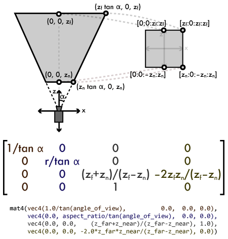
From these variables, we can come up with a general function to construct a projection matrix for any view frustum. The math is a little hairy; I'll describe what it does in broad strokes. With the camera at the origin, we can project the z axis directly to w axis values. In an affine transformation matrix, the bottom row is always set to [0 0 0 1]. This leaves the w axis unchanged. Changing this bottom row will cause the x, y, or z axis values to project onto the w axis, giving a perspective effect along the specified axis. In our case, setting that last row to [0 0 1 0] projects the z axis value directly to the perspective scale on w.
We'll then need to remap the range on the z axis from zn to zf so that it projects into the space between the near (–1) and far (1) planes of projection space. Taking the effect of the w coordinate into account, we'll have to map into the range from –zn (which with a w coordinate of zn will project to –1) to zf (which with a w coordinate that's also zf will project to 1). We do this by translating and scaling the z axis to fit this new range. The angle of view is determined by how much we scale the x and y axes. A scale of one gives a 45° angle of view; shrinking the axes gives a wider field of view, and growing them gives a narrower field, inversely proportional to the tangent of the angle of view. So that our output isn't distorted, we also scale the y axis proportionally to the aspect ratio (r) of the viewport.
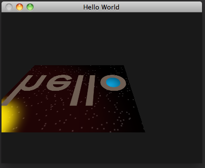
Let's write one last shader using the view frustum matrix function. We'll translate the rectangle to set it 3 units in front of us. In addition to rotating around the x axis, we'll also change the translation over time to set it moving in a circle left to right and toward and away from us. Here's the code, from view-frustum-rotation.v.glsl:
#version 110

uniform float timer;

attribute vec4 position;

varying vec2 texcoord;
varying float fade_factor;

mat4 view_frustum(
    float angle_of_view,
    float aspect_ratio,
    float z_near,
    float z_far
) {
    return mat4(
        vec4(1.0/tan(angle_of_view),           0.0, 0.0, 0.0),
        vec4(0.0, aspect_ratio/tan(angle_of_view),  0.0, 0.0),
        vec4(0.0, 0.0,    (z_far+z_near)/(z_far-z_near), 1.0),
        vec4(0.0, 0.0, -2.0*z_far*z_near/(z_far-z_near), 0.0)
    );
}

mat4 scale(float x, float y, float z)
{
    return mat4(
        vec4(x,   0.0, 0.0, 0.0),
        vec4(0.0, y,   0.0, 0.0),
        vec4(0.0, 0.0, z,   0.0),
        vec4(0.0, 0.0, 0.0, 1.0)
    );
}

mat4 translate(float x, float y, float z)
{
    return mat4(
        vec4(1.0, 0.0, 0.0, 0.0),
        vec4(0.0, 1.0, 0.0, 0.0),
        vec4(0.0, 0.0, 1.0, 0.0),
        vec4(x,   y,   z,   1.0)
    );
}

mat4 rotate_x(float theta)
{
    return mat4(
        vec4(1.0,         0.0,         0.0, 0.0),
        vec4(0.0,  cos(timer),  sin(timer), 0.0),
        vec4(0.0, -sin(timer),  cos(timer), 0.0),
        vec4(0.0,         0.0,         0.0, 1.0)
    );
}

void main()
{
    gl_Position = view_frustum(radians(45.0), 4.0/3.0, 0.5, 5.0)
        * translate(cos(timer), 0.0, 3.0+sin(timer))
        * rotate_x(timer)
        * scale(4.0/3.0, 1.0, 1.0)
        * position;
    texcoord = position.xy * vec2(0.5) + vec2(0.5);
    fade_factor = sin(timer) * 0.5 + 0.5;
}
And this is what we get:
Matrix multiplication is by far the most common operation in a 3d rendering pipeline. The rotation, scaling, translation, and frustum matrices we've covered are the basic structures that make 3d graphics happen. With these fundamentals covered, we're now ready to start building 3d scenes. If you want to learn more about 3d math, the book 3d Math Primer for Graphics and Game Development gives excellent in-depth coverage beyond the basics I've touched on here.
In this chapter, I've been demonstrating matrix math by writing code completely within the vertex shader. Constructing our matrices in the vertex shader will cause the matrices to be redundantly calculated for every single vertex. For this simple four-vertex program, it's not a big deal; I stuck to GLSL because it has great support for matrix math built into the language, and demonstrating both the concepts of matrix math and a hoary C math library would make things even more confusing. Unfortunately, OpenGL provides no matrix or vector math through the C API, so we'd need to use a third-party library, such as libSIMDx86, to perform this math outside of shaders. In a real program with potentially thousands of vertices, the extra matrix math overhead in the vertex shader will add up. Projection matrices generally apply to an entire scene and only need to be recalculated when the window is resized or the screen resolution changed, and model-view matrices usually change only between frames and apply to sets of vertices, so it is more efficient to precalculate these matrices and feed them to the shader as uniforms or attributes. This is how we'll do things from now on.
In the next chapter, we'll leave this lame "hello world" program behind and write a program that renders a more sophisticated 3d scene. In the process, we'll look at the next most important aspect of 3d rendering after transformation and projection: lighting.